In this chapter, you will understand and demonstrate knowledge in the following areas:
| Displaying data from multiple tables | |
| Group functions and their uses | |
| Using subqueries | |
| Using runtime variables |
The previous chapter covered the basics of select statements in order to get the user started with SQL and with Oracle. Data selection is probably the most common operation executed by users of an Oracle database. There are many advanced techniques for selecting the data the user needs to understand. This understanding includes mastery of such tasks as ad-hoc reporting, screen data population, and other types of work that requires selecting data. This chapter will cover the advanced topics of Oracle data selection. The following areas of SQL select statements will be discussed. The first area of understanding discussed in this chapter is the table join. The chapter will cover how users can write select statements to access data from more than one table. The discussion will also cover how the user can create joins that capture data from different tables even when the information in the two tables does not correspond completely. Finally, the use of table self-joins will be discussed. The chapter also introduces the group by clause used in select statements and group functions. Use of the subquery is another area covered in this chapter. The writing of subqueries and different situations where subqueries are useful is presented. Finally, specification and use of variables is presented. The material in this chapter will complete the user’s knowledge of data selection and also comprises 22 percent of OCP Exam 1.
In this section, you will cover the following areas related to displaying data from multiple tables:
| Select statements to join data from more than one table | |
| Creating outer joins | |
| Joining a table to itself |
The typical database contains many tables. Some smaller databases may have only a dozen or so tables, while other databases may have hundreds. The common factor, however, is that no database has just one table that contains all data that the user will need. Oracle recognizes that the user may want data that resides in multiple tables drawn together in some meaningful way. In order to allow the user to have that data all in one place, Oracle allows the user to perform table joins. A table join is when data from one table is associated with data from another table according to a common column that appears in both tables. This column is called a foreign key. Foreign keys between two tables create a relationship between the two tables that is referred to as referential integrity.
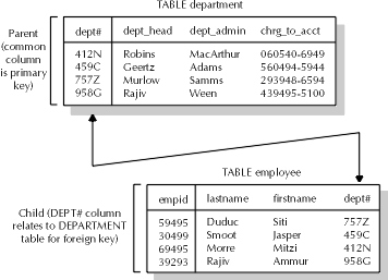
Foreign keys work in the following way. If a column appears in two tables, a foreign key relationship can be defined between them if one of the columns appears as part of a primary key in one of the tables. A primary key is used in a table to identify the uniqueness of each row in a table. The table in which the column appears as a primary key is referred to as the parent table, while the column that references the other table in the relationship is often called the child table. Figure 2-1 demonstrates how the relationship may work in a database.
Parent (common column is primary key)
Child (DEPT# column relates to DEPARTMENT table by foreign key)
Figure 1: Parent and child tables with foreign-key relationships
When a foreign-key relationship exists between several tables, then it is possible to merge the data in each table with data from another table to invent new meaning for the data in Oracle. This technique is accomplished with the use of a table join. As described in the last chapter, a select statement can have three parts: the select clause, the from clause, and the where clause. The select clause is where the user will list the column names he or she wants to view data from, along with any single-row functions and/or column aliases. The from clause gives the names of the tables from which the data would be selected. So far, data from only one table at a time has been selected. In a table join, two or more tables are named to specify the joined data. The final clause is the where clause, which contains comparison operations that will filter out the unwanted data from what the user wants to see. The comparison operations in a table join statement have another purpose—to describe how the data between two tables should be joined together.
SELECT a.antique_name, a.antique_cost,
a.storage_box_number, b.box_name, b.box_location
FROM antique a, storage_box b
WHERE a.antique_name in (‘VICTROLA’,’CAMERA’,’RADIO’)
AND a.storage_box_number = b.storage_box_number;
A.ANTIQUE_N A.ANTIQ A.STOR B.BOX_NAME B.BOX_LOCATION
----------- ------- ------ ---------- --------------
VICTROLA 150.00 3 ALPHA-3
ALPHA BLDG
CAMERA 75.00 4
ALPHA-4 ALPHA BLDG
RADIO 200.00 4
ALPHA-4 ALPHA BLDG
Many important things are happening in this sample statement, the most fundamental of which is the table join. The from clause in this statement is the clearest indication that a table join statement is taking place. In this statement, the from clause contains two table names, each of which is followed by a letter. Table ANTIQUE in this example is followed by the letter A, while table STORAGE_BOX is followed by the letter B. This display demonstrates an interesting concept in Oracle—not only can the columns in a select statement have aliases, but the tables named in the from clause can have an aliases as well. Table aliases have an important use in a table join statement, as given evidence in both the select and the where clauses of this example statement.
Often, tables with columns in common will have the same name for those columns. This common name can lead to ambiguity when the Oracle SQL processing mechanism attempts to parse the statement and resolve all database object names. If each column isn’t linked to the particular tables identified in the from clause, Oracle will return an error. By specifying an alias for each table in the from clause, and then preceding each column in the database with the alias, the user can avoid ambiguity in his or her SQL statements while also avoiding the need to type out a table name each time a column is specified. The aliases, therefore, aren’t necessary, but they do reduce the number of characters the user has to type each time a column is specified. The following code block illustrates the extra coding necessary when referencing columns if table aliases aren’t used.
SELECT antique_name, antique_cost,
antique.storage_box_number, box_name, box_location
FROM antique, storage_box
WHERE antique_name in (‘VICTROLA’,’CAMERA’,’RADIO’)
AND antique.storage_box_number = storage_box.storage_box_number;
ANTIQUE_NAM ANTIQUE ANTIQU BOX_NAME BOX_LOCATION
----------- ------- ------ -------- ------------
VICTROLA 150.00 3 ALPHA-3
ALPHA BLDG
CAMERA 75.00 4
ALPHA-4 ALPHA BLDG
RADIO 200.00 4
ALPHA-4 ALPHA BLDG
As mentioned, eliminating ambiguity can be accomplished either by specifying the full table name before any column that appears in both tables or with the use of aliases. Remember also that neither the alias nor the full table name need be specified before a column that appears in only one table specified by the from clause. Ambiguity is only produced when the column appears in two or more of the tables specified in the from clause.
The next area to cover in creating queries that join data from one table to data from another table is the mechanism by which the join takes place. That mechanism is the use of comparison operations in the where clause of the statement. The where clause of the statement generally must include one comparison that links the data in one column of one table to the data from the same column in the other table. Without this link, all data from both tables is generated as output from the query in something referred to as a Cartesian product.
There are two possibilities available in order to link the data from one table column number to another. The alternatives are to perform equality comparisons or to perform inequality comparisons. The type of comparison used to produce the joined data often translates into the name of the join operation itself. In the situation where the tables are being joined based on an equality statement in the where clause, the join itself is often referred to as an "inner" join, or as an equijoin. An inner join will return data where the value in one column in one table equals the value in the column of the other table. In the situation where the tables are being joined based on a inequality statement in the where clause, typically the data returned may have less meaning unless a range of data is specified and the actual link between the two tables is an equality statement.
SELECT antique_name, antique_cost,
antique.storage_box_number, box_name, box_location
FROM antique, storage_box
WHERE antique_name IN (‘VICTROLA’,’CAMERA’,’RADIO’)
AND antique.storage_box_number < storage_box.storage_box_number;
ANTIQUE_NAM ANTIQUE ANTIQU BOX_NAME BOX_LOCATION
----------- ------- ------ -------- ------------
VICTROLA 150.00 3 ALPHA-1
ALPHA BLDG
VICTROLA 150.00 3 ALPHA-2
ALPHA BLDG
VICTROLA 150.00 3 ALPHA-3
ALPHA BLDG
VICTROLA 150.00 3 ALPHA-4
ALPHA BLDG
CAMERA 75.00 4
ALPHA-1 ALPHA BLDG
CAMERA 75.00 4
ALPHA-2 ALPHA BLDG
CAMERA 75.00 4
ALPHA-3 ALPHA BLDG
CAMERA 75.00 4
ALPHA-4 ALPHA BLDG
RADIO 200.00 4
ALPHA-1 ALPHA BLDG
RADIO 200.00 4
ALPHA-2 ALPHA BLDG
RADIO 200.00 4
ALPHA-3 ALPHA BLDG
RADIO 200.00 4
ALPHA-4 ALPHA BLDG
How does Oracle determine what data should be returned by this query? When Oracle tries to evaluate the second clause in the and statement, it may look at the data in the ANTIQUE table, one at a time, and determine which values in the storage box tables have a greater values set for STORAGE_BOX_NUMBER. If the value for that column in the first row of ANTIQUE is 2, then there may be several rows in STORAGE_BOX that have STORAGE_BOX_NUMBER set to values greater than 2. However, in the second row of the ANTIQUE table, the value set to the STORAGE_BOX_NUMBER might be 1, returning almost every row in the STORAGE_BOX table because the values for STORAGE_BOX_NUMBER in that table are all greater than 1. The point of this example is to illustrate that when an inequality operation is specified as part of the where clause joining data from one table to another, there is no way to guarantee that the inequality operation will be satisfied for all values in the column for both tables. There is also a high possibility that the data returned by an inequality join will look suspiciously like a Cartesian product.
A better alternative for drawing data from a table that satisfies an inequality operation but does not produce a Cartesian product is to specify the inequality operation outside the comparison that produces the join as shown below:
SELECT antique_name, antique_cost,
antique.storage_box_number, box_name, box_location
FROM antique, storage_box
WHERE box_location in (‘VICTROLA’,’CAMERA’,’RADIO’)
AND antique.storage_box_number = storage_box.storage_box_number
AND antique.storage_box_number > 3;
ANTIQUE_NAM ANTIQUE ANTIQU BOX_NAME BOX_LOCATION
----------- ------- ------ -------- ------------
CAMERA 75.00 4
ALPHA-4 ALPHA BLDG
RADIO 200.00 4
ALPHA-4 ALPHA BLDG
This select statement will produce all results joined properly using the equality operation to link the rows of two tables in an inner join, while also satisfying the less-than comparison needed to obtain data for only those storage boxes less than box #2. In general, it is best to specify an equality operation for the two columns linking the tables for the join, followed by an inequality operation on the same column in one of the tables to filter the number of rows that will be linked in the join.
Generally speaking, the query used to produce a table join must contain the right number of equality operations to avoid a Cartesian product. If the number of tables to be joined equals N, the user should remember to include at least N-1 equality conditions in the select statement so that each column in each table that exists in another table is referenced at least once.
Tip: For N joined tables, you need at least N-1 join conditions in the select statement in order to avoid a Cartesian product.
In some cases, however, the user needs some measure of inequality on the joined columns of a table join operation in order to produce the data required in the return set. Consider, for example, that the user in this antique store wanted to see all Victrolas not in storage boxes as well as those that are boxed. One limitation of "inner" join or equijoin statements is that they will not return data from either table unless there is a common value in both columns for both tables on which to make the join.
SELECT antique_name, antique_cost,
antique.storage_box_number, box_name, box_location
FROM antique, storage_box
WHERE box_location = ‘VICTROLA’
AND antique.storage_box_number = storage_box.storage_box_number;
ANTIQUE_NAM ANTIQUE ANTIQU BOX_NAME BOX_LOCATION
----------- ------- ------ -------- ------------
VICTROLA 150.00 3 ALPHA-3
ALPHA BLDG
Notice that in this example, only Victrolas that have corresponding storage box entries in the STORAGE_BOX table will be included in the return set. In an attempt to obtain a list of Victrolas that are not boxed, the user then issues the following nonjoin query:
SELECT antique_name, antique_cost
FROM antique;
ANTIQUE_NAM ANTIQUE
----------- -------
VICTROLA 150.00
VICTROLA 90.00
VICTROLA 45.00
This query is a little closer to the mark, returning data on antique Victrolas regardless of whether or not they are boxed, but the user still needs to see storage box information for those Victrolas that are boxed. In order to force the join to return data from one table even if there is no corresponding record in the other table, the user can specify an outer join operation. The inner join statement above can be modified in the following way to show records in the ANTIQUE table that have no corresponding record in the STORAGE_BOX table:
SELECT antique_name, antique_cost,
antique.storage_box_number, box_name, box_location
FROM antique, storage_box
WHERE box_location = ‘VICTROLA’
AND antique.storage_box_number = storage_box.storage_box_number (+);
ANTIQUE_NAM ANTIQUE ANTIQU BOX_NAME BOX_LOCATION
----------- ------- ------ -------- ------------
VICTROLA 150.00 3 ALPHA-3
ALPHA BLDG
VICTROLA 90.00
VICTROLA 75.00
Join statements such as these, which produce result sets that are "outside" the join criteria as well as inside it, are often referred to as "outer" joins. Notice the special (+) marker at the end of the comparison that forms the join. This marker denotes which column can have null data corresponding to the non-null values in the other table. In the example above, the outer join marker is on the side of the STORAGE_BOX table, meaning that data in the ANTIQUE table can correspond either to values in STORAGE_BOX or to null if there is no corresponding value in STORAGE_BOX.
In special situations, it may be necessary for the user to perform a join using only one table. This task can be useful in certain cases where there is a possibility that some slight difference exists between two rows that would otherwise be duplicate records. If the user wants to perform a self join on a table, the user should utilize the table alias method described earlier in the chapter to specify the same table for Oracle to understand that a self join is being performed.
The following example of a self join shows how to use this technique properly. For the example, assume that there is a table called TEST_RESULTS on which users at various locations administer a test for employees of a large corporation. The test is designed to determine if a given employee is ready for promotion. If an employee fails the test, he or she must wait a full year before taking the test again. It is discovered that there is a bug in the system that allowed some employees to circumvent the rule by taking the test at a different location. Now, management wants to find out which employees have taken the test more than once in the past year. The columns in the TEST_RESULTS table are listed as follows: EMPID, LOCATION, DATE, and SCORE. In order to determine if an employee has taken the test twice in the last year, the user could issue the following SQL select that uses self join techniques:
SELECT a.empid, a.location, a.date, b.location, b.date
FROM test_results a, test_results b
WHERE a.empid = b.empid
AND a.location <> b.location
AND a.date > sysdate-365
AND b.date > sysdate-365;
A.EMPID A.LOCATION A.DATE B.LOCATION B.DATE
------- ---------- --------- ---------- ---------
94839 St. John 04-NOV-97 Wendt
03-JAN-98
04030 Stridberg 27-JUN-97 Wendt 03-AUG-97
59393 St. John 20-SEP-97 Wendt
04-OCT-97
The output from this self join shows that three employees took the test in different locations within the last 12 months. The clause used to determine DATE highlights the flexibility inherent in Oracle’s internal method for storing DATE datatypes and sysdate as numbers representing the number of days since the beginning of the Julian calendar. The storage method Oracle uses allows the user to perform simple mathematical operations on dates to obtain other dates without worrying about taking into account factors like the number of days in months between the old date and new, whether the year in question is a leap year, etc.
Those users who must perform self joins on tables should be extremely cautious about doing so in order to avoid performance issues or Cartesian products. The required number of equality operations is usually at least two in the situation of self joins, simply because only using one equality condition usually does not limit the output of a self join to the degree that the output must be limited in order to obtain meaningful information.
Tip: The number of equality operations required in the where clause of a self join should usually be greater than or equal to 2.
It should be stated that a self join typically requires a long time to execute, because Oracle must necessarily read all data for each table twice sequentially. Ordinarily, Oracle will read data from two different tables to perform the join, but since the operation in this case is a self join, all data comes from one table. Also, the user must be careful with self joins to ensure that a Cartesian product is not produced. Without a proper comparison operation set up in the where clause, the user may wind up with many copies of every row in the table returned, which will certainly run for a long time and produce a lot of unnecessary output.
In this section, you will cover the following areas related to group functions and their uses:
| Identifying available group functions | |
| Using group functions | |
| Using the group by clause | |
| Excluding group data with having |
After the single-value functions of the last chapter, there are some commonly used group functions. A group function allows the user to perform a data operation on several values in a column of data as though the column was one collective group of data. These functions are called group functions also, because they are often used in a special clause of select statements called a group by clause. A more complete discussion of the group by clause appears in the second discussion of this section.
A list of important group functions appears in this discussion. An important advantage group functions offer over single-row functions is that group functions can operate on several rows at a time. This advantage allows functions to be used that calculate figures like averages and standard deviation. The list of available group functions appears below:
| avg(x) | Average for all x column values returned by the select statement |
| count(x) | A sum of all rows returned by the select statement for column x |
| max(x) | The maximum value in column x for all rows returned by the select statement |
| min(x) | The minimum value in column x for all rows returned by the select statement |
| stddev(x) | The standard deviation for all values in column x in all rows returned by select statements |
| sum(x) | The sum of all values in column x in all rows returned by the select statement |
| variance(x) | The variance for all values in column x in all rows returned by select statements |
Examples of output from each of the following group functions appear over the next several pages. Since these functions require the use of several rows of data, the EMP table from the previous chapter will be used frequently. To refresh the discussion, the EMP table appears in Table 3-1.
| Empid | Lastname | Fname | Salary |
| 39334 | Smith | Gina | 75,000 |
| 49539 | Qian | Lee | 90,000 |
| 60403 | Harper | Rod | 45,000 |
| 02039 | Walla | Rajendra | 60,000 |
| 49392 | Spanky | Stacy | 100,000 |
Table 1: The EMP Table
The first function considered is the avg( ) function. The avg( ) function takes the values for a column on rows returned by the query and calculates the average value for that column. Based on the data from the table above, the avg( ) function on the SALARY column produces the following result:
SELECT AVG(salary)FROM EMP;
AVG(salary)
-----------
74000
The second grouping function that will be illustrated is the count( ) function. This function is bound to become the cornerstone of any Oracle professional’s repertoire. The count( ) function returns a row count for the table given certain column names and/or select criteria. It is worth learning the best way to use this command. There are many different ways to use the count( ) function, three of which are listed below. Note that the fastest way to execute count( ) is to pass a value that resolves quickly in the SQL processing mechanism. Some values that resolve quickly are integers and the ROWID pseudocolumn.
SELECT COUNT(*), COUNT, COUNT(rowid)The asterisk (*) in the query above is a wildcard variable that indicates all columns in all rows in the table. For better performance, this wildcard should not generally be used because the Oracle SQL processing mechanism must first resolve all column names in the table, a step that is unnecessary if one is simply trying to count rows. Notice that one of these examples uses the special pseudocolumn called ROWID. A ROWID is a special value that uniquely identifies each row. In the next unit covering OCP Exam 2, the use of ROWID to identify the location on disk of row data will be explained. Each row in a table has one unique ROWID. The ROWID is not actually part of the table; rather, ROWID is a piece of information stored internally within Oracle. Thus, it is considered a "pseudocolumn."
The next pair of grouping functions to be covered are the max( )/min( ) functions. The max( ) function determines the largest value for the column passed, while min( ) determines the smallest value for the column passed.
SELECT MAX(salary), MIN(salary) FROM EMP;
MAX(salary) MIN(salary)
----------- -----------
100000 45000
Another group function details the variance( ) of all values in a column. The variance of a set of numbers represents a measure of variability–-the mean squared deviation from the expected value for the set.
SELECT VARIANCE(salary) FROM EMP;
VARIANCE(salary)
----------------
492500000
Related to variance( ) is the next example in this section–-the stddev( ) function. It produces the standard deviation for values in the column specified. Standard deviation is the square root of the variance for the set–-a measure of variability. The number produced represents the margin of variance or error for a set of numbers.
SELECT STDDEV(salary) FROM EMP;
STDDEV(salary)
--------------
22192.341
The final group function is used commonly in simple accounting reports. The sum( ) function gives the total of all values in a column.
SELECT SUM(salary) FROM EMP;
SUM(salary)
-----------
370000
In general, the group functions will operate on columns of datatype NUMBER because many of the functions they represent in mathematics are numeric operations. For example, it makes little sense to take the standard deviation for a set or 12 words, unless the user wants to take the standard deviation of the length of those words by combining the use of the length( ) function with the stddev( ) function. There is one notable exception to this general rule, though--that exception is the count( ) function. The count( ) function will operate on a column of any datatype.
Sometimes it gives more meaning to the output of a select statement to collect data into logical groupings. For example, to perform calculations on the populations of several cities in America, the user may issue a query against all records in the CITIES table. The select statements, such as ones containing order by, may work well for specific queries against particular cities in this table, such as listing data in order based on an alphabetized list of cities and states such as the SQL statement listed:
SELECT state, city, population
FROM cities
ORDER BY state, city;
STATE CITY
POPULATION
--------------- -------------- ----------
ALABAMA AARDVARK
12,560
ALABAMA BARNARD
176,000
…
Consider the following example, however. There arises a situation where a user wants to perform specific calculations on the cities in each state separately. For example, assume the user wants to find out the average city population for each of the states listed on the table. This select statement works fine for producing the raw data the user needs to calculate the average city population for each state; however, there is an easier way for the user to determine this information based on usage of the group by clause in SQL statements.
SELECT state, AVG(population)
FROM CITIES
GROUP BY state
ORDER BY state;
STATE AVG(POPULA
----------------- ----------
ALABAMA 49494
ALASKA 14349
NEW YORK 85030
ARIZONA 35003
CALIFORNIA 65040
…
The group by clause in this example saves the user from performing a great deal of work by hand. Instead, Oracle shoulders most of the work and outputs to the user only the results he or she needs. The group by clause works well in many situations where a user wants to report calculations on data according to groups or categories. However, the user should be careful to always place the column on which the group by clause will group the data first in the list of columns specified by the select clause. If the columns being grouped using the group by clause are not in the same sequential order and first in the list of columns selected, then the user could encounter one of the most problematic Oracle error messages: ORA-00937 – Not a single group set function.
To illustrate the usage of group by in another example, assume that the user now wants to calculate the average salary for all employees in a corporation by department. The EMP table contains the following columns: EMPID, LASTNAME, FIRSTNAME, SALARY, and DEPT. However, in addition to obtaining the average employee salary by department, the user wants the information in order from highest average salary to lowest.
SELECT dept, AVG(salary)
FROM emp
GROUP BY dept
ORDER BY avg(salary) DESC;
DEPT AVG(SALARY)
---- -----------
201B 103020
594C 94030
493W 71039
201C 50403
In this example, the order by clause was combined with the group by clause to create a special order for the output. This order gives the data some additional meaning to the user who requested its display. The user is not limited to grouping data by only one selected column, either. If the user desires, more than one column can be used in the group by statement–-provided that the order of columns specified in the select clause of the query matches the order of columns specified in the group by clause. The following example illustrates proper usage of group by with more than one column specified. It assumes the addition of a column, COUNTRY, which names the country containing the city. Notice that the columns named in the group by clause are in the same order as they are named in the select clause. It often must be set up in this way in order to avoid errors.
SELECT country, state, AVG(population)
FROM cities
GROUP BY country, state;
One initial problem encountered when using the group by statement is that once the data is grouped, the user must then analyze the data returned by the group by statement in order to determine which groups are relevant and which are not. It is sometimes useful to the user to weed out unwanted data. For example, in the final query from the previous section, suppose the user only wanted to see which departments paid an average salary of $80,000 per year. In effect, the user is attempting to put a where clause on the group by clause.
This effect can be gained with the use of a special clause in Oracle called having. This clause acts as a modified where clause that only applies to the resultant rows generated by the group by expression. Consider the application of the modifications above to the query of employee salary by department. If the user wants to view only those departments whose employees make an average of $80,000 or more, the user may want to issue the following query. The having clause in this case is used to eliminate the departments whose average salary is under $80,000. Notice that this selectivity cannot easily be accomplished with an ordinary where clause, because the where clause is selective to the precision of individual rows while the user requires selectivity for eliminating groups of rows.
SELECT dept, AVG(salary)
FROM emp
GROUP BY dept HAVING avg(salary)>80000
ORDER BY avg(salary) DESC;
DEPT AVG(SALARY)
---- -----------
201B 103020
705B 94030
In this query, the user has successfully limited output on the group by rows by using the having clause. But the having clause need not be limited by some arbitrary number that the user must key in manually. In addition to performing a comparison operation on a constant value, the having clause can perform a special operation to derive the required data with the use of a subquery. A subquery is another SQL query embedded within the overarching query being executed by the user that derives some special value required by a part of the entire query. Subqueries are useful to incorporate into select statements when there is a need for valid value data that the user does not actually know the value of, but knows the manner in which to obtain it. Take, for example, that the user in this situation would like to compare her salary with that of the rest of the departments in the company. Unfortunately, the user doesn’t know her salary, but the user does know her empid is 49394. In order to execute the following query again, only modified according to the current needs of the user, the following statement can be utilized:
SELECT dept, AVG(salary)
FROM emp
GROUP BY dept HAVING AVG(salary)>(SELECT salary FROM emp WHERE empid=49394)
ORDER BY avg(salary) DESC;
DEPT AVG(SALARY)
---- -----------
201B 103020
569A 96120
In this section, you will cover the following topics related to using subqueries:
| Nested subqueries | |
| Subqueries in other DML situations | |
| Putting data in order with subqueries |
The usage of subqueries need not be limited to the having clause of a group by statement. The power of subqueries to determine unknown criteria based on known methods for obtaining it can be used in many different ways. Of particular importance in using subqueries is incorporating them properly into comparison operations of the where clause. There are several different ways to include subqueries in where statements. The most common method used is through the equality comparison operation, or with the in comparison, which is in itself similar to a case statement offered in many programming languages in that the equality can be established with one element in the group. Another useful item for inclusion of a subquery in the where clause of a select statement is the exists clause. When a user specifies the exists operation in a where clause, the user must include a subquery that satisfies the exists operation. If the subquery returns data, then the exists operation returns TRUE. If not, the exists operation returns FALSE. These and other uses for subqueries will be discussed shortly.
Subqueries can be used to obtain search criteria for select statements. The way subqueries work is as follows. The where clause in a select statement has one or more comparison operations. Each comparison operation can contain the name of a column on the left side and a given search method to obtain unknown data on the right side by means of a subquery.
SELECT empid, dept, salary
FROM emp
WHERE dept = (select dept from emp where empid = 78483);
The portion of the SQL statement above that is highlighted is the subquery portion of the statement. On one side is the DEPT column, on which a comparison will be based to determine the result dataset. On the other side is the unknown search criteria, defined by the subquery. At the time this select statement is submitted, Oracle will process the subquery first in order to resolve all unknown search criteria, then feed that resolved criteria to the outer query. The outer query then can resolve the dataset it is supposed to return.
Similar to the outer query, the subquery itself can contain subqueries. This process is known as nested subqueries. Consider the following example. There is a user trying to determine the salary of employees in the same department as an employee who has submitted an expensive invoice for payment on the company’s relocation expenditure system. The tables involved in this select statement are the EMP table, which has been described, and the INVOICE table, which consists of the following columns: INVOICE_NUMBER, EMPID, INVOICE_AMT, and PAY_DATE. The only information the user has about the employee they are looking for is the invoice number the employee submitted for relocation expenses, which is 5640.
SELECT e.empid, e.salary
FROM emp e
WHERE e.dept =
(SELECT dept FROM emp WHERE empid =
(SELECT empid FROM invoice WHERE invoice_number = 5640));
In the statement above, there are two subqueries, the subquery to the main select statement highlighted in bold, and the nested subquery in italics. Each subquery produces unknown criteria to fulfill the main search occurring in the select statement, the first producing the department information and the second producing the employee ID for the person submitting the invoice. These two details are crucial for completing the select statement, yet the data is unknown to the user at the time the select statement is issued. Oracle must first resolve the innermost nested subquery in italics to resolve the next level. After that, Oracle will resolve the subquery level in bold to resolve the outermost level of the select statement issued.
Subqueries can be nested to a surprisingly deep level. The rule of thumb used to be that the user could nest 16 or more subqueries into a select statement. In reality, the number of nested subqueries can be far higher. However, if a user needs to nest more than five subqueries, he or she may want to consider writing the query in PL/SQL or in a programming language like PRO*C or PRO*COBOL or some other programming language that allows embedded SQL statements and cursors. At the very least, the user may want to consider rewriting a query that makes heavy use of subqueries into a query that performs extensive join operations as well. The reason these recommendations are made is because database performance degrades substantially after about that level when processing nested subqueries on all but the most powerful database servers and mainframes. At the very least, the user should check carefully to ensure that there are no performance issues within the nested query that may slow down database performance significantly.
The discussion above covered many areas of using subqueries in data manipulation statements. However, that discussion barely scratches the surface on the power of subqueries. A subquery can be used for complicated step-by-step joins of data that use data from one subquery to feed into the processing of its immediate parent. However, subqueries also allow the user to "jump" subquery levels to perform incredibly complex, almost counterintuitive processing that necessarily must involve some discussion of a programming concept known as variable scope. For those users not familiar with the term, variable scope refers to the availability or "viewability" of data in certain variables at certain times.
Sometimes a variable has a local scope. That is to say that the variable can only be seen when the current block of code is being executed. For the purposes of this discussion, the user can consider the columns in comparison operations named in subqueries to be variables whose "scope" is local to the query. Additionally, there is another type of scope, called global scope. In addition to a variable having local scope within the subquery where it appears, the variable also has global scope in all subqueries to that query. In the previous select statement example, all variables or columns named in comparison operations in the outermost select operation are local to that operation and global to all nested subqueries, given in bold and italics. Additionally, all columns in the subquery detailed in bold are local to that query and global to the subquery listed in italics. Columns named in the query in italics are local to that query only; since there are no subqueries to it, the columns in that query cannot be global. The nested query example from the previous discussion is featured in Figure 2-2.
Outermost query in select statement; DEPT column is global to all subqueries
First subquery; EMPID is local to the subquery but global to the following subquery
Innermost subquery; invoice_number is local to this query only
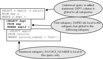
Figure 2: Nested subqueries and variable scope
In certain cases, it may be useful for a subquery to refer to a global column value rather than a local one to obtain result data. The subquery architecture of Oracle allows the user to refer to global variables in subqueries as well as local ones to produce more powerful queries. An example of this type of global scope usage, sometimes also referred to as correlated subqueries, is as follows. Assume that there is a recruiter for a national consulting firm who wants to find people in Minneapolis who are proficient in Oracle DBA skills. Furthermore, the recruiter only wants to see the names and home cities for people who are certified Oracle DBAs. The recruiter has at her disposal a nationwide resume search system with several tables. These tables include one called CANDIDATE, which contains the candidate ID, candidate name, salary requirement and current employer. Another table in this example is called SKILLS, where the candidate ID is matched with the skill the candidate possesses. A third table, called COMPANIES, contains the names and home cities for companies that the consulting firm tries to draw their talent from. In order to find the names and locations of people who possess the abilities the recruiter requires, the recruiter may issue the following select statement against the national recruiting database:
SELECT candidate_id, name, employer
FROM candidate
WHERE candidate_id IN
(SELECT candidate_id FROM skills
WHERE skill_type = ‘ORACLE DBA’ AND certified = ‘YES’)
AND employer IN
(SELECT employer FROM companies WHERE city = ‘MINNEAPOLIS’);
CANDIDATE_ID NAME EMPLOYER
------------ -------- --------------
60549 DURNAM TransCom
This query produces the result set the recruiter is looking for. However, there is one anomaly about this query, which is highlighted in bold in the preceding code block. The first subquery, which selects candidate IDs based on a search for specific skills, performs its operation on the SKILLS table. Notice that there is a reference to the EMPLOYER column from the CANDIDATE table in this subquery. This column is not present in the SKILLS table, but nonetheless it can be referred to by the subquery because the columns from the CANDIDATE table are global to all subqueries, because the CANDIDATE table is in the outermost query of the select statement. Notice in the last subquery the use of the in keyword. Recall from the discussion in Chapter 2 that the in operation allows the user to identify a set of values, any of which the column named in the in clause can equal in order to be part of the result set. Thus, if the where clause of the select statement contains and number in (1,2,3), that means only the rows whose value in the NUMBER column are equal to 1, 2, or 3 will be part of the result set.
Another complicated possibility offered by subqueries is the use of the exists operation. Mentioned earlier, exists allows the user to specify the results of a select statement according to a special subquery operation. This exists operation returns TRUE or FALSE based on whether or not the subquery obtains data when it runs. An example of the usage for the exists subquery is related to a previous example of the relocation expenditure tracking system. To refresh the discussion, the tables involved in this system are the EMP table, which has been described, and the INVOICE table, which consists of the following columns: INVOICE_NUMBER, EMPID, INVOICE_AMT, and PAY_DATE. Let’s assume that the user wants to identify all the departments that have employees that have incurred relocation expenses in the past year.
SELECT distinct e.dept
FROM emp e
WHERE EXISTS
(SELECT i.empid FROM invoice i
WHERE i.empid = e.empid AND i.pay_date > SYSDATE-365);
There are several new things that are worthy of note in this select statement. The first point to be made is that global scope variables are again incorporated in the subquery to produce meaningful results from that code. The second point to make is more about the general nature of exists statements. Oracle will go through every record in the EMP table to see if the EMPID matches that of a row in the INVOICE table. If there is a matching invoice, then the exists criteria is met and the department ID is added to the list of departments that will be returned. If not, then the exists criteria is not met and the record is not added to the list of departments that will be returned.
Notice that there is one other aspect of this query that has not been explained—the distinct keyword highlighted in bold in the select column clause of the outer portion of the query. This special keyword identifies a filter that Oracle will put on the data returned from the exists subquery. When distinct is used, Oracle will return only one row for a particular department, even if there are several employees in that department that have submitted relocation expenses within the past year. This distinct operation is useful for situations when the user wants a list of unique rows but anticipates that the query may return duplicate rows. The distinct operation removes duplicate rows from the result set before displaying that result to the user.
As with other types of select statements, those statements that involve subqueries may also require some semblance of order in the data that is returned to the user. In the examples of subquery usage in the previous discussion, there may be a need to return the data in a particular order based on the columns selected by the outermost query. In this case, the user may simply want to add in the usage of the order by clause. The previous example of selecting the departments containing relocated employees could be modified as follows to produce the required department data in a particular order required by the user:
SELECT distinct e.dept
FROM emp e
WHERE EXISTS
(SELECT i.empid FROM invoice i
WHERE i.empid = e.empid AND i.pay_date > SYSDATE-365)
ORDER BY dept;
As in using the order by statement in other situations, the data returned from a statement containing a subquery and the order by clause can be sorted into ascending or descending order. Furthermore, the user can incorporate order into the data returned by the subquery.
SELECT distinct e.dept
FROM emp e
WHERE EXISTS
(SELECT i.empid FROM invoice I
WHERE i.empid = e.empid AND i.pay_date > SYSDATE-365)
ORDER BY i.empid;
In this example, the data returned from the exists subquery will appear in ascending order. However, since the fundamental point of the exists subquery is to determine whether the data exists that the subquery is looking for, it is probably considered overkill to return data in order from most subqueries. However, for those times when it might be useful, the user should understand that the potential does exist for returning data from a subquery in order.
In another example, the points made before about global and local scope will be reinforced. A recruiter from the national consulting firm mentioned earlier tries to issue the following select statement, similar to the original one discussed with that example:
SELECT candidate_id, name, employer
FROM candidate
WHERE candidate_id IN
(SELECT candidate_id FROM skills
WHERE employer IN
(SELECT employer FROM companies
WHERE city = ‘MINNEAPOLIS’))
ORDER BY skill_type;
When the recruiter attempts to issue the preceding select statement, Oracle will execute the statement without error because the column specified by the order by clause need not be part of the column list in the select column list of the outermost select statement. However, within a subquery it is possible for the user to create order based on the column "variables" from the outer query. Order, then, can only be made on the columns local or global to the query on which the order by clause is placed.
What special clause is used to determine the order of output in a select statement containing a subquery?
In this section, you will cover the following topics related to using runtime variables
| Entering variables at run time | |
| Automatic definition of runtime variables | |
| Accept: another way to define variables |
SQL is an interpreted language. That is, there is no "executable code" other than the statement the user enters into the command line. At the time that statement is entered, Oracle’s SQL processing mechanism works on obtaining the data and returning it to the user. When Oracle is finished returning the data, it is ready for the user to enter another statement. This interactive behavior is typical of interpreted programming languages.
SELECT name, salary, dept
FROM emp
WHERE empid = 40539;
NAME SALARY DEPT
-------- ------- ----
DURNAP 70560 450P
In the statement above, the highlighted comparison operation designates that the data returned from this statement must correspond to the EMPID value specified. If the user were to run this statement again, the data returned would be exactly the same, provided that no portion of the record had been changed by the user issuing the query or any other user on the database. However, Oracle’s interpretive SQL processing mechanism need not have everything defined for it at the time the user enters a SQL statement. In fact, there are features within the SQL processing mechanism of Oracle that allow the user to identify a specific value to be used for the execution of the query as a runtime variable. This feature permits some flexibility and reusability of SQL statements.
Consider, for example, the situation where a user must pull up data for several different employees manually for the purpose of reviewing some aspect of their data. Rather than rekeying the entire statement in with the EMPID value hard-coded into each statement, the user can substitute a variable specification that forces Oracle to prompt the user to enter a data value in order to let Oracle complete the statement. The statement above that returned data from the EMP table based on a hard-coded EMPID value can now be rewritten as the following query that allows the user to reuse the same code again and again with different values set for EMPID:
SELECT name, salary, dept
FROM emp
WHERE empid = &empid;
Enter value for empid: 40539
Old 3: WHERE empid = &empid;
New 3: WHERE empid = 40539;
NAME SALARY DEPT
------ ------- ----
DURNAP 70560 450P
After completing execution, the user now has the flexibility to rerun that same query, except now that user can specify a different EMPID without having to reenter the entire statement. Notice that a special ampersand (&) character precedes the name of the variable that will be specified at run time. The actual character can be changed with the set define command at the prompt. The user can reexecute the statement containing a runtime variable declaration by using the slash(/) command at the prompt in SQL*Plus.
Enter value for empid: 99706
Old 3: WHERE empid = &empid;
New 3: WHERE empid = 99706;
NAME SALARY DEPT
------- ------- ----
MCCALL 103560 795P
This time, the user enters another value for the EMPID, and Oracle searches for data in the table based on the new value specified. This activity will go on as listed above until the user enters a new SQL statement. Notice that Oracle provides additional information back to the user after a value is entered for the runtime variable. The line as it appeared before is listed as the old value, while below the new value is presented as well. This presentation allows the user to know what data was changed by his or her input.
In some cases, however, it may not be useful to have the user entering new values for a runtime variable every time the statement executes. For example, assume that there is some onerous reporting process that a user must perform weekly on every person in a company. A great deal of value is added to the process by having a variable that can be specified at run time because the user can now simply reexecute the same statement over and over again, with new EMPID values each time. However, even this improvement is not streamlining the process as much as the user would like. Instead of running the statement over and over again with new values specified, the user could create a script that contained the SQL statement, preceded by a special statement that defined the input value automatically and triggered the execution of the statement automatically as well. Some basic reporting conventions will be presented in this example, such as spool. This command is used to designate to the Oracle database that all output generated by the following SQL activity should be redirected to an output file named after the parameter following spool:
SPOOL emp_info.out;
DEFINE VAR_EMPID = 34030
SELECT name, salary, dept
FROM emp
WHERE empid = &var_empid
UNDEFINE VAR_EMPID
DEFINE VAR_EMPID = 94059
SELECT name, salary, dept
FROM emp
WHERE empid = &var_empid
When the user executes the statements in the script above, the time spent actually keying in values for the variables named in the SQL select statement is eliminated with the define statement. Notice, however, that in between each execution of the SQL statement there is a special statement using a command called undefine. In Oracle, the data that is defined with the define statement as corresponding to the variable will remain defined for the entire session unless the variable is undefined. By undefining a variable, the user allows another define statement to reuse the variable in another execution of the same or a different statement.
After executing a few example SQL statements that incorporate runtime variables, the user will notice that Oracle’s method for identifying input, though not exactly cryptic, is fairly nonexpressive.
SELECT name, salary, dept
FROM emp
WHERE empid = &empid
AND dept = ‘&dept’;
Enter value for &empid: 30403
Old 3: WHERE empid = &empid
New 3: WHERE empid = 30403
Enter value for &dept: 983X
Old 4: WHERE dept = ‘&dept’
New 4: WHERE dept = ‘983X’
NAME SALARY DEPT
-------- -------- ----
TIBBINS 56700 983X
The user need not stick with Oracle’s default messaging to identify the need for input from a user. Instead, the user can incorporate into scripted SQL statements another method for the purpose of defining runtime variables. This other method allows the creator of the script to define a more expressive message that the user will see when Oracle prompts for input data. The name of the command that provides this functionality is the accept command. In order to use the accept command in a runtime SQL environment, the user can create a script in the following way. Assume for the sake of example that the user has created a script called name_sal_dept.sql, into which the following SQL statements are placed:
ACCEPT var_empid PROMPT ‘Enter the Employee ID Now:’
ACCEPT var_dept PROMPT ‘Enter the Employee Department Now:’
SELECT name, salary, dept
FROM emp
WHERE empid = &var_empid
AND dept = ‘&var_dept’
At this point, the user can run the script at the prompt using the following command syntax:
SQL> @emp_sal_dept
or
SQL> start emp_sal_dept.sql
Oracle will then execute the contents of the script. When Oracle needs to obtain the runtime value for the variables that the user identified in the SQL statement and with the accept statement, Oracle will use the prompt the user defined with the prompt clause of the accept statement.
SQL> @emp_sal_dept
Enter the Employee ID Now: 30403
SELECT name, salary, dept
FROM emp
WHERE empid = &var_empid
AND dept = ‘&var_dept’
Old 3: WHERE dept = ‘&dept’
New 3: WHERE empid = 30403
Enter the Employee Dept Now: 983X
SELECT name, salary, dept
FROM emp
WHERE empid = 30403
AND dept = ‘&var_dept’
Old 4: WHERE dept = ‘&dept’
New 4: WHERE dept = ‘983X’
NAME SALARY DEPT
-------- ------- ----
TIBBINS 56700 983X
Using the accept command can be preferable to Oracle’s default output message in situations where the user wants to define a more accurate or specific prompt, or the user wants more output to display as the values are defined. In either case, the accept command can work well. Oracle offers a host of options for making powerful and complex SQL statements possible with runtime variables. These options covered can be used for both interactive SQL data selection and for SQL scripts.
This chapter continues the discussion presented last chapter of using the select statement to obtain data from the Oracle database. The select statements have many powerful features that allow the user to accomplish many tasks. Those features include joining data from multiple tables, grouping data output together and performing data operations on the groups of data, creating select statements that can use subqueries to obtain criteria that is unknown (but the method for obtaining it is known), and using variables that accept values at run time. Together, these areas comprise the advanced usage of SQL select statements. The material in this chapter comprises 22 percent of information questioned on OCP Exam 1.
The first area discussed in this chapter is how data from multiple tables can be joined together to create new meaning. Data in a table can be linked if there is a common or shared column between the two tables. This shared column is often referred to as a foreign key. Foreign keys establish a relationship between two tables that is referred to as a parent/child relationship. The parent table is typically the table in which the common column is defined as a primary key, or the column by which uniqueness is identified for rows in the table. The child table is typically the table in which the column is not the primary key, but refers to the primary key in the parent table.
There are two types of joins. One of those types is the "inner" join, also known as an equijoin. An inner join is a data join based on equality comparisons between common columns of two or more tables. An "outer" join is a nonequality join operation that allows the user to obtain output from a table even if there is no corresponding data for that record in the other table.
Joins are generated by using select statements in the following way. First, the columns desired in the result set are defined in the select clause of the statement. Those columns may or may not be preceded with a table definition, depending on whether or not the column appears in more than one table. If the common column is named differently in each table, then there is no need to identify the table name along with the column name, as Oracle will be able to distinguish which table the column belongs to automatically. However, if the column name is duplicated in two or more tables, then the user must specify which column he or she would like to obtain data from, since Oracle must be able to resolve any ambiguities clearly at the time the query is parsed. The columns from which data is selected are named in the from clause, and may optionally be followed by a table alias. A table alias is similar in principle to a column alias, which was discussed in the last chapter. The where clause of a join statement specifies how the join is performed. An inner join is created by specifying the two shared columns in each table in an equality comparison. An outer join is created in the same way, with an additional special marker placed by the column specification of the "outer" table, or the table in which there need not be data corresponding to rows in the other table for that data in the other table to be returned. That special marker is indicated by a (+). Finally, a table may be joined to itself with the use of table aliases. This activity is often done to determine if there are records in a table with slightly different information from rows that otherwise are duplicate rows.
Another advanced technique for data selection in Oracle databases is the use of grouping functions. Data can be grouped together in order to provide additional meaning to the data. Columns in a table can also be treated as a group in order to perform certain operations on them. These grouping functions often perform math operations such as averaging values or obtaining standard deviation on the dataset. Other group functions available on groups of data are max( ), min( ), sum( ), and count( ).
One common grouping operation performed on data for reporting purposes is a special clause in select statements called group by. This clause allows the user to segment output data and perform grouping operations on it. There is another special operation associated with grouping that acts as a where clause for which to limit the output produced by the selection. This limiting operation is designated by the having keyword. The criteria for including or excluding data using the having clause can be identified in one of two ways. Either criterion can be a hard-coded value or it can be based on the results of a select statement embedded into the overarching select statement. This embedded selection is called a subquery.
Another advanced function offered by select statements is the use of subqueries in the where clause of the select statement. A select statement can have 16 or more nested subqueries in the where clause, although it is not generally advisable to do so based on performance. Subqueries allow the user to specify unknown search criteria for the comparisons in the where clause as opposed to using strictly hard-coded values. Subqueries also illustrate the principle of data scope in SQL statements by virtue of the fact that the user can specify columns that appear in the parent query, even when those columns do not appear in the table used in the subquery.
Another use of subqueries can be found in association with a special operation that can be used in the where clause of a select statement. The name of this special operation is exists. This operation produces a TRUE or FALSE value based on whether or not the related subquery produces data. The exists clause is a popular option for users to incorporate subqueries into their select statements.
Output from the query can be placed into an order specified by the user with the assistance of the order by clause. However, the user must make sure that the columns in the order by clause are the same as those actually listed by the outermost select statement. The order by clause can also be used in subqueries; however, since the subqueries of a select statement are usually used to determine a valid value for searching or as part of an exists clause, the user should be more concerned about the existence of the data than the order in which data is returned from the subquery. Therefore, there is not much value added to using the order by clause in subqueries.
One final advanced technique covered in this chapter is the specification of variables at run time. This technique is especially valuable in order to provide reusability in a data selection statement. In order to denote a runtime variable in SQL, the user should place a variable name in the comparison operation the user wants to specify a runtime value for. The name of that variable in the select statement should be preceded with a special character to denote it as a variable. By default, this character is an ampersand (&). However, the default variable specification character can be changed with the use of the set define command at the prompt.
Runtime variables can be specified for SQL statements in other ways as well. The define command can be used to identify a runtime variable for a select statement automatically. After being defined and specified in the define command, a variable is specified for the entire session or until it is altered with the undefine command. In this way, the user can avoid the entire process of having to input values for the runtime variables. The final technique covered in this chapter on select statements is the usage of accept to redefine the text displayed for the input prompt. More cosmetic than anything else, accept allows the user to display a more direct message than the Oracle default message for data entry.
| Select statements that obtain data from more than one table and merge the data together are called joins. | |
| In order to join data from two tables, there must be a common column. | |
| A common column between two tables can create a foreign key, or link, from one table to another. This condition is especially true if the data in one of the tables is part of the primary key, or the column that defines uniqueness for rows on a table. | |
| A foreign key can create a parent/child relationship between two tables. | |
| One type of join is the inner join, or equijoin. An equijoin operation is based on an equality operation linking the data in common columns of two tables. | |
| Another type of join is the outer join. An outer join returns data in one table even when there is no data in the other table. | |
| The "other" table in the outer join operation is called the outer table. | |
| The common column that appears in the outer table of the join must have a special marker next to it in the comparison operation of the select statement that creates the table. | |
| The outer join marker is as follows: (+). | |
| Common columns in tables used in join operations must be preceded either with a table alias that denotes the table in which the column appears, or else the entire table name if the column name is the same in both tables. | |
| The data from a table can be joined to itself. This technique is useful in determining if there are rows in the table that have slightly different values but are otherwise duplicate rows. | |
| Table aliases must be used in self join select statements. | |
| Data output from table select statements can be grouped together according to criteria set by the query. | |
| A special clause exists to assist the user in grouping data together. That clause is called group by. | |
| There are several grouping functions that allow the user to perform operations on data in a column as though the data were logically one variable. | |
| The grouping functions are max( ), min( ), sum( ), avg( ), stddev( ), variance( ), and count( ). | |
| These grouping functions can be applied to the column values for a table as a whole or for subsets of column data for rows returned in group by statements. | |
| Data in a group by statement can be excluded or included based on a special set of where criteria defined specifically for the group in a having clause. | |
| The data used to determine the having clause can either be specified at run time by the query or by a special embedded query, called a subquery, which obtains unknown search criteria based on known search methods. | |
| Subqueries can be used in other parts of the select statement to determine unknown search criteria as well. Including subqueries in this fashion typically appears in the where clause. | |
| Subqueries can use columns in comparison operations that are either local to the table specified in the subquery or use columns that are specified in tables named in any parent query to the subquery. This usage is based on the principles of variable scope as presented in this chapter. | |
| Data can be returned from statements containing subqueries with the order by clause. | |
| It is not typically recommended for users to use order by in the subquery itself, as the subquery is generally designed to test a valid value or produce an intermediate dataset result. Order is usually not important for these purposes. | |
| Variables can be set in a select statement at run time with use of runtime variables. A runtime variable is designated with the ampersand character (&) preceding the variable name. | |
| The special character that designates a runtime variable can be changed using the set define command. | |
| A command called define can identify a runtime variable value to be picked up by the select statement automatically. | |
| Once defined, the variable remains defined for the rest of the session or until undefined by the user or process with the undefine command. | |
| A user can also modify the message that prompts the user to input a variable value. This activity is performed with the accept command. |